Note

From Ray 2.6.0 onwards, RLlib is adopting a new stack for training and model customization, gradually replacing the ModelV2 API and some convoluted parts of Policy API with the RLModule API. Click here for details.

算法#

Tip

Check out the environments page to learn more about different environment types.

Available Algorithms - Overview#

Algorithm	Frameworks	Discrete Actions	Continuous Actions	Multi-Agent	Model Support	Multi-GPU
A2C	tf + torch	Yes +parametric	Yes	Yes	+RNN, +LSTM auto-wrapping, +Attention, +autoreg	A2C: tf + torch
A3C	tf + torch	Yes +parametric	Yes	Yes	+RNN, +LSTM auto-wrapping, +Attention, +autoreg	No
AlphaZero	torch	Yes +parametric	No	No		No
APPO	tf + torch	Yes +parametric	Yes	Yes	+RNN, +LSTM auto-wrapping, +Attention, +autoreg	tf + torch
ARS	tf + torch	Yes	Yes	No		No
Bandits (TS & LinUCB)	torch	Yes +parametric	No	Yes		No
BC	tf + torch	Yes +parametric	Yes	Yes	+RNN	torch
CQL	tf + torch	No	Yes	No		tf + torch
CRR	torch	Yes +parametric	Yes	Yes		torch
DDPG	tf + torch	No	Yes	Yes		torch
APEX-DDPG	tf + torch	No	Yes	Yes		torch
DreamerV3	tf	Yes	Yes	No	+RNN (GRU-based by default)	tf
Dreamer	torch	No	Yes	No	+RNN	torch
DQN, Rainbow	tf + torch	Yes +parametric	No	Yes		tf + torch
APEX-DQN	tf + torch	Yes +parametric	No	Yes		torch
ES	tf + torch	Yes	Yes	No		No
IMPALA	tf + torch	Yes +parametric	Yes	Yes	+RNN, +LSTM auto-wrapping, +Attention, +autoreg	tf + torch
LeelaChessZero	torch	Yes +parametric	No	Yes		torch
MAML	tf + torch	No	Yes	No		torch
MARWIL	tf + torch	Yes +parametric	Yes	Yes	+RNN	torch
MBMPO	torch	No	Yes	No		torch
PG	tf + torch	Yes +parametric	Yes	Yes	+RNN, +LSTM auto-wrapping, +Attention, +autoreg	tf + torch
PPO	tf + torch	Yes +parametric	Yes	Yes	+RNN, +LSTM auto-wrapping, +Attention, +autoreg	tf + torch
R2D2	tf + torch	Yes +parametric	No	Yes	+RNN, +LSTM auto-wrapping, +autoreg	torch
SAC	tf + torch	Yes	Yes	Yes		torch
SlateQ	tf + torch	Yes (multi-discr. slates)	No	No		torch
TD3	tf + torch	No	Yes	Yes		torch

Multi-Agent only Methods

Algorithm	Frameworks	Discrete Actions	Continuous Actions	Multi-Agent	Model Support
QMIX	torch	Yes +parametric	No	Yes	+RNN
MADDPG	tf	Yes	Partial	Yes
Parameter Sharing	Depends on bootstrapped algorithm
Fully Independent Learning	Depends on bootstrapped algorithm
Shared Critic Methods	Depends on bootstrapped algorithm

Exploration-based plug-ins (can be combined with any algo)

Algorithm	Frameworks	Discrete Actions	Continuous Actions	Multi-Agent	Model Support
Curiosity	tf + torch	Yes +parametric	No	Yes	+RNN

Offline#

Behavior Cloning (BC; derived from MARWIL implementation)#

[paper] [implementation]

Our behavioral cloning implementation is directly derived from our MARWIL implementation, with the only difference being the beta parameter force-set to 0.0. This makes BC try to match the behavior policy, which generated the offline data, disregarding any resulting rewards. BC requires the offline datasets API to be used.

Tuned examples: CartPole-v1

BC-specific configs (see also common configs):

Critic Regularized Regression (CRR)#

[paper] [implementation]

CRR is another offline RL algorithm based on Q-learning that can learn from an offline experience replay. The challenge in applying existing Q-learning algorithms to offline RL lies in the overestimation of the Q-function, as well as, the lack of exploration beyond the observed data. The latter becomes increasingly important during bootstrapping in the bellman equation, where the Q-function queried for the next state’s Q-value(s) does not have support in the observed data. To mitigate these issues, CRR implements a simple and yet powerful idea of “value-filtered regression”. The key idea is to use a learned critic to filter-out the non-promising transitions from the replay dataset. For more details, please refer to the paper (see link above).

Tuned examples: CartPole-v1, Pendulum-v1

Conservative Q-Learning (CQL)#

[paper] [implementation]

In offline RL, the algorithm has no access to an environment, but can only sample from a fixed dataset of pre-collected state-action-reward tuples. In particular, CQL (Conservative Q-Learning) is an offline RL algorithm that mitigates the overestimation of Q-values outside the dataset distribution via conservative critic estimates. It does so by adding a simple Q regularizer loss to the standard Bellman update loss. This ensures that the critic does not output overly-optimistic Q-values. This conservative correction term can be added on top of any off-policy Q-learning algorithm (here, we provide this for SAC).

RLlib’s CQL is evaluated against the Behavior Cloning (BC) benchmark at 500K gradient steps over the dataset. The only difference between the BC- and CQL configs is the bc_iters parameter in CQL, indicating how many gradient steps we perform over the BC loss. CQL is evaluated on the D4RL benchmark, which has pre-collected offline datasets for many types of environments.

Tuned examples: HalfCheetah Random, Hopper Random

CQL-specific configs (see also common configs):

Monotonic Advantage Re-Weighted Imitation Learning (MARWIL)#

[paper] [implementation]

MARWIL is a hybrid imitation learning and policy gradient algorithm suitable for training on batched historical data. When the beta hyperparameter is set to zero, the MARWIL objective reduces to vanilla imitation learning (see BC). MARWIL requires the offline datasets API to be used.

Tuned examples: CartPole-v1

MARWIL-specific configs (see also common configs):

Model-free On-policy RL#

Asynchronous Proximal Policy Optimization (APPO)#

[paper] [implementation] We include an asynchronous variant of Proximal Policy Optimization (PPO) based on the IMPALA architecture. This is similar to IMPALA but using a surrogate policy loss with clipping. Compared to synchronous PPO, APPO is more efficient in wall-clock time due to its use of asynchronous sampling. Using a clipped loss also allows for multiple SGD passes, and therefore the potential for better sample efficiency compared to IMPALA. V-trace can also be enabled to correct for off-policy samples.

Tip

APPO is not always more efficient; it is often better to use standard PPO or IMPALA.

../_images/impala-arch.svg — APPO architecture (same as IMPALA)#

Tuned examples: PongNoFrameskip-v4

APPO-specific configs (see also common configs):

Decentralized Distributed Proximal Policy Optimization (DD-PPO)#

[paper] [implementation] Unlike APPO or PPO, with DD-PPO policy improvement is no longer done centralized in the algorithm process. Instead, gradients are computed remotely on each rollout worker and all-reduced at each mini-batch using torch distributed. This allows each worker’s GPU to be used both for sampling and for training.

Tip

DD-PPO is best for envs that require GPUs to function, or if you need to scale out SGD to multiple nodes. If you don’t meet these requirements, standard PPO will be more efficient.

../_images/ddppo-arch.svg — DD-PPO architecture (both sampling and learning are done on worker GPUs)#

Tuned examples: CartPole-v1, BreakoutNoFrameskip-v4

DDPPO-specific configs (see also common configs):

Proximal Policy Optimization (PPO)#

[paper] [implementation] PPO’s clipped objective supports multiple SGD passes over the same batch of experiences. RLlib’s multi-GPU optimizer pins that data in GPU memory to avoid unnecessary transfers from host memory, substantially improving performance over a naive implementation. PPO scales out using multiple workers for experience collection, and also to multiple GPUs for SGD.

Tip

If you need to scale out with GPUs on multiple nodes, consider using decentralized PPO.

../_images/ppo-arch.svg — PPO architecture#

Tuned examples: Unity3D Soccer (multi-agent: Strikers vs Goalie), Humanoid-v1, Hopper-v1, Pendulum-v1, PongDeterministic-v4, Walker2d-v1, HalfCheetah-v2, {BeamRider,Breakout,Qbert,SpaceInvaders}NoFrameskip-v4

Atari results: more details

Atari env	RLlib PPO @10M	RLlib PPO @25M	Baselines PPO @10M
BeamRider	2807	4480	~1800
Breakout	104	201	~250
Qbert	11085	14247	~14000
SpaceInvaders	671	944	~800

Scalability: more details

MuJoCo env	RLlib PPO 16-workers @ 1h	Fan et al PPO 16-workers @ 1h
HalfCheetah	9664	~7700

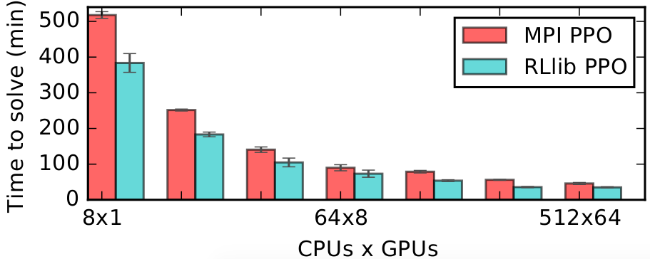
../_images/ppo.png — RLlib’s multi-GPU PPO scales to multiple GPUs and hundreds of CPUs on solving the Humanoid-v1 task. Here we compare against a reference MPI-based implementation.#

PPO-specific configs (see also common configs):

Importance Weighted Actor-Learner Architecture (IMPALA)#

[paper] [implementation] In IMPALA, a central learner runs SGD in a tight loop while asynchronously pulling sample batches from many actor processes. RLlib’s IMPALA implementation uses DeepMind’s reference V-trace code. Note that we do not provide a deep residual network out of the box, but one can be plugged in as a custom model. Multiple learner GPUs and experience replay are also supported.

Tuned examples: PongNoFrameskip-v4, vectorized configuration, multi-gpu configuration, {BeamRider,Breakout,Qbert,SpaceInvaders}NoFrameskip-v4

Atari results @10M steps: more details

Atari env	RLlib IMPALA 32-workers	Mnih et al A3C 16-workers
BeamRider	2071	~3000
Breakout	385	~150
Qbert	4068	~1000
SpaceInvaders	719	~600

Scalability:

Atari env	RLlib IMPALA 32-workers @1 hour	Mnih et al A3C 16-workers @1 hour
BeamRider	3181	~1000
Breakout	538	~10
Qbert	10850	~500
SpaceInvaders	843	~300

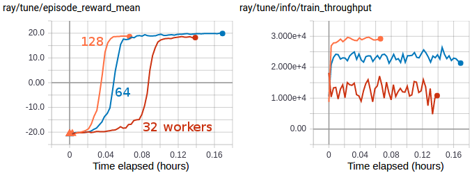
../_images/impala.png — Multi-GPU IMPALA scales up to solve PongNoFrameskip-v4 in ~3 minutes using a pair of V100 GPUs and 128 CPU workers. The maximum training throughput reached is ~30k transitions per second (~120k environment frames per second).#

IMPALA-specific configs (see also common configs):

Advantage Actor-Critic (A2C)#

[paper] [implementation] A2C scales to 16-32+ worker processes depending on the environment and supports microbatching (i.e., gradient accumulation), which can be enabled by setting the microbatch_size config. Microbatching allows for training with a train_batch_size much larger than GPU memory.

../_images/a2c-arch.svg — A2C architecture#

Tuned examples: Atari environments

Tip

Consider using IMPALA for faster training with similar timestep efficiency.

Atari results @10M steps: more details

Atari env	RLlib A2C 5-workers	Mnih et al A3C 16-workers
BeamRider	1401	~3000
Breakout	374	~150
Qbert	3620	~1000
SpaceInvaders	692	~600

A2C-specific configs (see also common configs):

Asynchronous Advantage Actor-Critic (A3C)#

[paper] [implementation] A3C is the asynchronous version of A2C, where gradients are computed on the workers directly after trajectory rollouts, and only then shipped to a central learner to accumulate these gradients on the central model. After the central model update, parameters are broadcast back to all workers. Similar to A2C, A3C scales to 16-32+ worker processes depending on the environment.

Tuned examples: PongDeterministic-v4

Tip

Consider using IMPALA for faster training with similar timestep efficiency.

A3C-specific configs (see also common configs):

Policy Gradients (PG)#

[paper] [implementation] We include a vanilla policy gradients implementation as an example algorithm.

Tuned examples: CartPole-v1

PG-specific configs (see also common configs):

Model-Agnostic Meta-Learning (MAML)#

[paper] [implementation]

RLlib’s MAML implementation is a meta-learning method for learning and quick adaptation across different tasks for continuous control. Code here is adapted from https://github.com/jonasrothfuss, which outperforms vanilla MAML and avoids computation of the higher order gradients during the meta-update step. MAML is evaluated on custom environments that are described in greater detail here.

MAML uses additional metrics to measure performance; episode_reward_mean measures the agent’s returns before adaptation, episode_reward_mean_adapt_N measures the agent’s returns after N gradient steps of inner adaptation, and adaptation_delta measures the difference in performance before and after adaptation. Examples can be seen here.

Tuned examples: HalfCheetahRandDirecEnv (Env, Config), AntRandGoalEnv (Env, Config), PendulumMassEnv (Env, Config)

MAML-specific configs (see also common configs):

Model-free Off-policy RL#

Distributed Prioritized Experience Replay (Ape-X)#

[paper] [implementation] Ape-X variations of DQN and DDPG (APEX_DQN, APEX_DDPG) use a single GPU learner and many CPU workers for experience collection. Experience collection can scale to hundreds of CPU workers due to the distributed prioritization of experience prior to storage in replay buffers.

../_images/apex-arch.svg — Ape-X architecture#

Tuned examples: PongNoFrameskip-v4, Pendulum-v1, MountainCarContinuous-v0, {BeamRider,Breakout,Qbert,SpaceInvaders}NoFrameskip-v4.

Atari results @10M steps: more details

Atari env	RLlib Ape-X 8-workers	Mnih et al Async DQN 16-workers
BeamRider	6134	~6000
Breakout	123	~50
Qbert	15302	~1200
SpaceInvaders	686	~600

Scalability:

Atari env	RLlib Ape-X 8-workers @1 hour	Mnih et al Async DQN 16-workers @1 hour
BeamRider	4873	~1000
Breakout	77	~10
Qbert	4083	~500
SpaceInvaders	646	~300

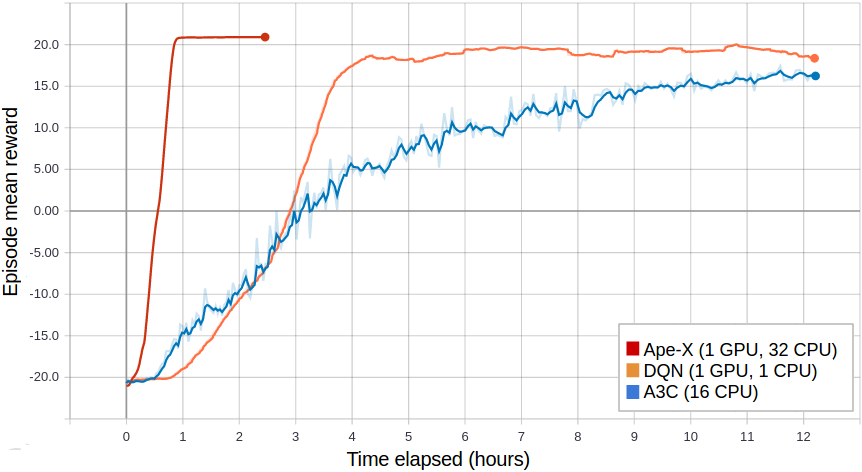
../_images/apex.png — Ape-X using 32 workers in RLlib vs vanilla DQN (orange) and A3C (blue) on PongNoFrameskip-v4.#

Ape-X specific configs (see also common configs):

Recurrent Replay Distributed DQN (R2D2)#

[paper] [implementation] R2D2 can be scaled by increasing the number of workers. All of the DQN improvements evaluated in Rainbow are available, though not all are enabled by default.

Tuned examples: Stateless CartPole-v1

Deep Q Networks (DQN, Rainbow, Parametric DQN)#

[paper] [implementation] DQN can be scaled by increasing the number of workers or using Ape-X. Memory usage is reduced by compressing samples in the replay buffer with LZ4. All of the DQN improvements evaluated in Rainbow are available, though not all are enabled by default. See also how to use parametric-actions in DQN.

../_images/dqn-arch.svg — DQN architecture#

Tuned examples: PongDeterministic-v4, Rainbow configuration, {BeamRider,Breakout,Qbert,SpaceInvaders}NoFrameskip-v4, with Dueling and Double-Q, with Distributional DQN.

Tip

Consider using Ape-X for faster training with similar timestep efficiency.

Hint

For a complete rainbow setup, make the following changes to the default DQN config: "n_step": [between 1 and 10], "noisy": True, "num_atoms": [more than 1], "v_min": -10.0, "v_max": 10.0 (set v_min and v_max according to your expected range of returns).

Atari results @10M steps: more details

Atari env	RLlib DQN	RLlib Dueling DDQN	RLlib Dist. DQN	Hessel et al. DQN
BeamRider	2869	1910	4447	~2000
Breakout	287	312	410	~150
Qbert	3921	7968	15780	~4000
SpaceInvaders	650	1001	1025	~500

DQN-specific configs (see also common configs):

Deep Deterministic Policy Gradients (DDPG)#

[paper] [implementation] DDPG is implemented similarly to DQN (below). The algorithm can be scaled by increasing the number of workers or using Ape-X. The improvements from TD3 are available as TD3.

Tuned examples: Pendulum-v1, MountainCarContinuous-v0, HalfCheetah-v2.

DDPG-specific configs (see also common configs):

Twin Delayed DDPG (TD3)#

[paper] [implementation] TD3 represents an improvement over DDPG. Its implementation is available in RLlib as TD3.

Tuned examples: TD3 Pendulum-v1, TD3 InvertedPendulum-v2, TD3 Mujoco suite (Ant-v2, HalfCheetah-v2, Hopper-v2, Walker2d-v2).

TD3-specific configs (see also common configs):

Soft Actor Critic (SAC)#

[original paper], [follow up paper], [discrete actions paper] [implementation]

RLlib’s soft-actor critic implementation is ported from the official SAC repo to better integrate with RLlib APIs. Note that SAC has two fields to configure for custom models: policy_model_config and q_model_config, the model field of the config will be ignored.

Tuned examples (continuous actions): Pendulum-v1, HalfCheetah-v3, Tuned examples (discrete actions): CartPole-v1

MuJoCo results @3M steps: more details

MuJoCo env	RLlib SAC	Haarnoja et al SAC
HalfCheetah	13000	~15000

SAC-specific configs (see also common configs):

Model-based RL#

DreamerV3#

[paper] [implementation]

DreamerV3 trains a world model in supervised fashion using real environment interactions. The world model’s objective is to correctly predict all aspects of the transition dynamics of the RL environment, which includes (besides predicting the correct next observations) predicting the received rewards as well as a boolean episode continuation flag. A “recurrent state space model” or RSSM is used to alternatingly train the world model (from actual env data) as well as the critic and actor networks, both of which are trained on “dreamed” trajectories produced by the world model.

DreamerV3 can be used in all types of environments, including those with image- or vector based observations, continuous- or discrete actions, as well as sparse or dense reward functions.

Tuned examples: Atari 100k, Atari 200M, DeepMind Control Suite

Pong-v5 results (1, 2, and 4 GPUs):

../_images/pong_1_2_and_4gpus.svg — Episode mean rewards for the Pong-v5 environment (with the “100k” setting, in which only 100k environment steps are allowed): Note that despite the stable sample efficiency - shown by the constant learning performance per env step - the wall time improves almost linearly as we go from 1 to 4 GPUs. **Left**: Episode reward over environment timesteps sampled. **Right**: Episode reward over wall-time.#

Atari 100k results (1 vs 4 GPUs):

../_images/atari100k_1_vs_4gpus.svg — Episode mean rewards for various Atari 100k tasks on 1 vs 4 GPUs. **Left**: Episode reward over environment timesteps sampled. **Right**: Episode reward over wall-time.#

DeepMind Control Suite (vision) results (1 vs 4 GPUs):

../_images/dmc_1_vs_4gpus.svg — Episode mean rewards for various Atari 100k tasks on 1 vs 4 GPUs. **Left**: Episode reward over environment timesteps sampled. **Right**: Episode reward over wall-time.#

Dreamer#

[paper] [implementation]

Dreamer is an image-only model-based RL method that learns by imagining trajectories in the future and is evaluated on the DeepMind Control Suite environments. RLlib’s Dreamer is adapted from the official Google research repo.

To visualize learning, RLlib Dreamer’s imagined trajectories are logged as gifs in TensorBoard. Examples of such can be seen here.

Tuned examples: Deepmind Control Environments

Deepmind Control results @1M steps: more details

DMC env	RLlib Dreamer	Danijar et al Dreamer
Walker-Walk	920	~930
Cheetah-Run	640	~800

Dreamer-specific configs (see also common configs):

Model-Based Meta-Policy-Optimization (MB-MPO)#

[paper] [implementation]

RLlib’s MBMPO implementation is a Dyna-styled model-based RL method that learns based on the predictions of an ensemble of transition-dynamics models. Similar to MAML, MBMPO metalearns an optimal policy by treating each dynamics model as a different task. Code here is adapted from https://github.com/jonasrothfuss/model_ensemble_meta_learning. Similar to the original paper, MBMPO is evaluated on MuJoCo, with the horizon set to 200 instead of the default 1000.

Additional statistics are logged in MBMPO. Each MBMPO iteration corresponds to multiple MAML iterations, and MAMLIter$i$_DynaTrajInner_$j$_episode_reward_mean measures the agent’s returns across the dynamics models at iteration i of MAML and step j of inner adaptation. Examples can be seen here.

Tuned examples (continuous actions): Pendulum-v1, HalfCheetah, Hopper, Tuned examples (discrete actions): CartPole-v1

MuJoCo results @100K steps: more details

MuJoCo env	RLlib MBMPO	Clavera et al MBMPO
HalfCheetah	520	~550
Hopper	620	~650

MBMPO-specific configs (see also common configs):

Derivative-free#

Augmented Random Search (ARS)#

[paper] [implementation] ARS is a random search method for training linear policies for continuous control problems. Code here is adapted from https://github.com/modestyachts/ARS to integrate with RLlib APIs.

Tuned examples: CartPole-v1, Swimmer-v2

ARS-specific configs (see also common configs):

Evolution Strategies (ES)#

[paper] [implementation] Code here is adapted from https://github.com/openai/evolution-strategies-starter to execute in the distributed setting with Ray.

Tuned examples: Humanoid-v1

Scalability:

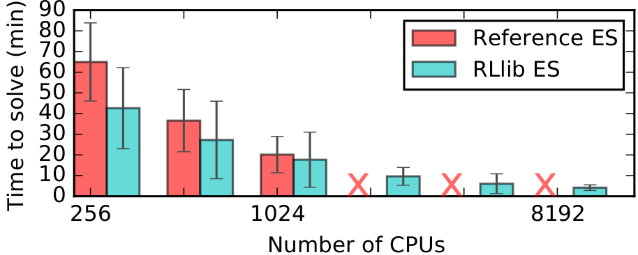
../_images/es.png — RLlib’s ES implementation scales further and is faster than a reference Redis implementation on solving the Humanoid-v1 task.#

ES-specific configs (see also common configs):

RL for recommender systems#

SlateQ#

[paper] [implementation]

SlateQ is a model-free RL method that builds on top of DQN and generates recommendation slates for recommender system environments. Since these types of environments come with large combinatorial action spaces, SlateQ mitigates this by decomposing the Q-value into single-item Q-values and solves the decomposed objective via mixing integer programming and deep learning optimization. SlateQ can be evaluated on Google’s RecSim environment. An RLlib wrapper for RecSim can be found here <.

RecSim environment wrapper: Google RecSim

SlateQ-specific configs (see also common configs):

Contextual Bandits#

The Multi-armed bandit (MAB) problem provides a simplified RL setting that involves learning to act under one situation only, i.e. the context (observation/state) and arms (actions/items-to-select) are both fixed. Contextual bandit is an extension of the MAB problem, where at each round the agent has access not only to a set of bandit arms/actions but also to a context (state) associated with this iteration. The context changes with each iteration, but, is not affected by the action that the agent takes. The objective of the agent is to maximize the cumulative rewards, by collecting enough information about how the context and the rewards of the arms are related to each other. The agent does this by balancing the trade-off between exploration and exploitation.

Contextual bandit algorithms typically consist of an action-value model (Q model) and an exploration strategy (epsilon-greedy, LinUCB, Thompson Sampling etc.)

RLlib supports the following online contextual bandit algorithms, named after the exploration strategies that they employ:

Linear Upper Confidence Bound (BanditLinUCB)#

[paper] [implementation] LinUCB assumes a linear dependency between the expected reward of an action and its context. It estimates the Q value of each action using ridge regression. It constructs a confidence region around the weights of the linear regression model and uses this confidence ellipsoid to estimate the uncertainty of action values.

Tuned examples: SimpleContextualBandit, UCB Bandit on RecSim. ParametricItemRecoEnv.

LinUCB-specific configs (see also common configs):

Linear Thompson Sampling (BanditLinTS)#

[paper] [implementation] Like LinUCB, LinTS also assumes a linear dependency between the expected reward of an action and its context and uses online ridge regression to estimate the Q values of actions given the context. It assumes a Gaussian prior on the weights and a Gaussian likelihood function. For deciding which action to take, the agent samples weights for each arm, using the posterior distributions, and plays the arm that produces the highest reward.

Tuned examples: SimpleContextualBandit, WheelBandit.

LinTS-specific configs (see also common configs):

Multi-agent#

QMIX Monotonic Value Factorisation (QMIX, VDN, IQN)#

[paper] [implementation] Q-Mix is a specialized multi-agent algorithm. Code here is adapted from https://github.com/oxwhirl/pymarl_alpha to integrate with RLlib multi-agent APIs. To use Q-Mix, you must specify an agent grouping in the environment (see the two-step game example). Currently, all agents in the group must be homogeneous. The algorithm can be scaled by increasing the number of workers or using Ape-X.

Tuned examples: Two-step game

QMIX-specific configs (see also common configs):

Multi-Agent Deep Deterministic Policy Gradient (MADDPG)#

[paper] [implementation] MADDPG is a DDPG centralized/shared critic algorithm. Code here is adapted from https://github.com/openai/maddpg to integrate with RLlib multi-agent APIs. Please check justinkterry/maddpg-rllib for examples and more information. Note that the implementation here is based on OpenAI’s, and is intended for use with the discrete MPE environments. Please also note that people typically find this method difficult to get to work, even with all applicable optimizations for their environment applied. This method should be viewed as for research purposes, and for reproducing the results of the paper introducing it.

MADDPG-specific configs (see also common configs):

Tuned examples: Multi-Agent Particle Environment, Two-step game

Shared Critic Methods#

[instructions] Shared critic methods are when all agents use a single parameter shared critic network (in some cases with access to more of the observation space than agents can see). Note that many specialized multi-agent algorithms such as MADDPG are mostly shared critic forms of their single-agent algorithm (DDPG in the case of MADDPG).

Tuned examples: TwoStepGame

Others#

Single-Player Alpha Zero (AlphaZero)#

[paper] [implementation] AlphaZero is an RL agent originally designed for two-player games. This version adapts it to handle single player games. The code can be scaled to any number of workers. It also implements the ranked rewards (R2) strategy to enable self-play even in the one-player setting. The code is mainly purposed to be used for combinatorial optimization.

Tuned examples: Sparse reward CartPole

AlphaZero-specific configs (see also common configs):

MultiAgent LeelaChessZero (LeelaChessZero)#

[source] [implementation] LeelaChessZero is an RL agent originally inspired by AlphaZero for playing chess. This version adapts it to handle a MultiAgent competitive environment of chess. The code can be scaled to any number of workers.

Tuned examples: tbd

LeelaChessZero-specific configs (see also common configs):

Curiosity (ICM: Intrinsic Curiosity Module)#

[paper] [implementation]

Tuned examples: Pyramids (Unity3D) (use --env Pyramids command line option) Test case with MiniGrid example (UnitTest case: test_curiosity_on_partially_observable_domain)

Activating Curiosity The curiosity plugin can be easily activated by specifying it as the Exploration class to-be-used in the main Algorithm config. Most of its parameters usually do not have to be specified as the module uses the values from the paper by default. For example:

config = ppo.DEFAULT_CONFIG.copy()
config["num_workers"] = 0
config["exploration_config"] = {
    "type": "Curiosity",  # <- Use the Curiosity module for exploring.
    "eta": 1.0,  # Weight for intrinsic rewards before being added to extrinsic ones.
    "lr": 0.001,  # Learning rate of the curiosity (ICM) module.
    "feature_dim": 288,  # Dimensionality of the generated feature vectors.
    # Setup of the feature net (used to encode observations into feature (latent) vectors).
    "feature_net_config": {
        "fcnet_hiddens": [],
        "fcnet_activation": "relu",
    },
    "inverse_net_hiddens": [256],  # Hidden layers of the "inverse" model.
    "inverse_net_activation": "relu",  # Activation of the "inverse" model.
    "forward_net_hiddens": [256],  # Hidden layers of the "forward" model.
    "forward_net_activation": "relu",  # Activation of the "forward" model.
    "beta": 0.2,  # Weight for the "forward" loss (beta) over the "inverse" loss (1.0 - beta).
    # Specify, which exploration sub-type to use (usually, the algo's "default"
    # exploration, e.g. EpsilonGreedy for DQN, StochasticSampling for PG/SAC).
    "sub_exploration": {
        "type": "StochasticSampling",
    }
}

Functionality RLlib’s Curiosity is based on “ICM” (intrinsic curiosity module) described in this paper here. It allows agents to learn in sparse-reward- or even no-reward environments by calculating so-called “intrinsic rewards”, purely based on the information content that is incoming via the observation channel. Sparse-reward environments are envs where almost all reward signals are 0.0, such as these [MiniGrid env examples here]. In such environments, agents have to navigate (and change the underlying state of the environment) over long periods of time, without receiving much (or any) feedback. For example, the task could be to find a key in some room, pick it up, find a matching door (matching the color of the key), and eventually unlock this door with the key to reach a goal state, all the while not seeing any rewards. Such problems are impossible to solve with standard RL exploration methods like epsilon-greedy or stochastic sampling. The Curiosity module - when configured as the Exploration class to use via the Algorithm’s config (see above on how to do this) - automatically adds three simple models to the Policy’s self.model: a) a latent space learning (“feature”) model, taking an environment observation and outputting a latent vector, which represents this observation and b) a “forward” model, predicting the next latent vector, given the current observation vector and an action to take next. c) a so-called “inverse” net, only used to train the “feature” net. The inverse net tries to predict the action taken between two latent vectors (obs and next obs).

All the above extra Models are trained inside the modified Exploration.postprocess_trajectory() call.

Using the (ever changing) “forward” model, our Curiosity module calculates an artificial (intrinsic) reward signal, weights it via the eta parameter, and then adds it to the environment’s (extrinsic) reward. Intrinsic rewards for each env-step are calculated by taking the euclidian distance between the latent-space encoded next observation (“feature” model) and the predicted latent-space encoding for the next observation (“forward” model). This allows the agent to explore areas of the environment, where the “forward” model still performs poorly (are not “understood” yet), whereas exploration to these areas will taper down after the agent has visited them often: The “forward” model will eventually get better at predicting these next latent vectors, which in turn will diminish the intrinsic rewards (decrease the euclidian distance between predicted and actual vectors).

RE3 (Random Encoders for Efficient Exploration)#

[paper] [implementation]

Examples: LunarLanderContinuous-v2 (use --env LunarLanderContinuous-v2 command line option) Test case with Pendulum-v1 example

Activating RE3 The RE3 plugin can be easily activated by specifying it as the Exploration class to-be-used in the main Algorithm config and inheriting the RE3UpdateCallbacks as shown in this example. Most of its parameters usually do not have to be specified as the module uses the values from the paper by default. For example:

config = sac.DEFAULT_CONFIG.copy()
config["env"] = "Pendulum-v1"
config["seed"] = 12345
config["callbacks"] = RE3Callbacks
config["exploration_config"] = {
    "type": "RE3",
     # the dimensionality of the observation embedding vectors in latent space.
     "embeds_dim": 128,
     "rho": 0.1, # Beta decay factor, used for on-policy algorithm.
     "k_nn": 50, # Number of neighbours to set for K-NN entropy estimation.
     # Configuration for the encoder network, producing embedding vectors from observations.
     # This can be used to configure fcnet- or conv_net setups to properly process any
     # observation space. By default uses the Policy model configuration.
     "encoder_net_config": {
         "fcnet_hiddens": [],
         "fcnet_activation": "relu",
     },
     # Hyperparameter to choose between exploration and exploitation. A higher value of beta adds
     # more importance to the intrinsic reward, as per the following equation
     # `reward = r + beta * intrinsic_reward`
     "beta": 0.2,
     # Schedule to use for beta decay, one of constant" or "linear_decay".
     "beta_schedule": 'constant',
     # Specify, which exploration sub-type to use (usually, the algo's "default"
     # exploration, e.g. EpsilonGreedy for DQN, StochasticSampling for PG/SAC).
     "sub_exploration": {
         "type": "StochasticSampling",
     }
}

Functionality RLlib’s RE3 is based on “Random Encoders for Efficient Exploration” described in this paper here. RE3 quantifies exploration based on state entropy. The entropy of a state is calculated based on its distance from K nearest neighbor states present in the replay buffer in the latent space (With this implementation, KNN is implemented using training samples from the same batch). The state entropy is considered as an intrinsic reward and for policy optimization added to the extrinsic reward when available. If the extrinsic reward is not available then the state entropy is used as “intrinsic reward” for unsupervised pre-training of the RL agent. RE3 further allows agents to learn in sparse-reward or even no-reward environments by using the state entropy as “intrinsic rewards”.

This exploration objective can be used with both model-free and model-based RL algorithms. RE3 uses a randomly initialized encoder to get the state’s latent representation, thus taking away the complexity of training the representation learning method. The encoder weights are fixed during the entire duration of the training process.

Fully Independent Learning#

[instructions] Fully independent learning involves a collection of agents learning independently of each other via single agent methods. This typically works, but can be less effective than dedicated multi-agent RL methods, since they do not account for the non-stationarity of the multi-agent environment.

Tuned examples: waterworld, multiagent-cartpole

Ray 2.7.2

算法

Contents

算法#

Available Algorithms - Overview#

Offline#

Behavior Cloning (BC; derived from MARWIL implementation)#

Critic Regularized Regression (CRR)#

Conservative Q-Learning (CQL)#

Monotonic Advantage Re-Weighted Imitation Learning (MARWIL)#

Model-free On-policy RL#

Asynchronous Proximal Policy Optimization (APPO)#

Decentralized Distributed Proximal Policy Optimization (DD-PPO)#

Proximal Policy Optimization (PPO)#

Importance Weighted Actor-Learner Architecture (IMPALA)#

Advantage Actor-Critic (A2C)#

Asynchronous Advantage Actor-Critic (A3C)#

Policy Gradients (PG)#

Model-Agnostic Meta-Learning (MAML)#

Model-free Off-policy RL#

Distributed Prioritized Experience Replay (Ape-X)#

Recurrent Replay Distributed DQN (R2D2)#

Deep Q Networks (DQN, Rainbow, Parametric DQN)#

Deep Deterministic Policy Gradients (DDPG)#

Twin Delayed DDPG (TD3)#

Soft Actor Critic (SAC)#

Model-based RL#

DreamerV3#

Dreamer#

Model-Based Meta-Policy-Optimization (MB-MPO)#

Derivative-free#

Augmented Random Search (ARS)#

Evolution Strategies (ES)#

RL for recommender systems#

SlateQ#

Contextual Bandits#

Linear Upper Confidence Bound (BanditLinUCB)#

Linear Thompson Sampling (BanditLinTS)#

Multi-agent#

Parameter Sharing#

QMIX Monotonic Value Factorisation (QMIX, VDN, IQN)#

Multi-Agent Deep Deterministic Policy Gradient (MADDPG)#

Shared Critic Methods#

Others#

Single-Player Alpha Zero (AlphaZero)#

MultiAgent LeelaChessZero (LeelaChessZero)#

Curiosity (ICM: Intrinsic Curiosity Module)#

RE3 (Random Encoders for Efficient Exploration)#

Fully Independent Learning#